Biotech Equity and Stock Option Valuation – A Deep Dive for Founders

Valuing a biotech venture is a bit like valuing a promising but precarious alchemical experiment – full of potential magic, but with plenty of risk and uncertainty. Founders often see a blockbuster cure in the making, while investors see a long, expensive road with many potholes. The result can be wildly different valuations for the same company. In fact, biotech companies with no current revenues can still command multi-billion-dollar valuations, as seen when Gilead paid nearly $12 billion for Kite Pharma’s pipeline CAR-T therapy in 2017. Conversely, public biotech markets can swing dramatically with clinical trial news, reflecting investors’ constantly shifting risk calculus.

In this comprehensive article, we’ll explore how to value biotech equity (for both private startups and public firms) using methods ranging from classic discounted cash flow to comparables to cutting-edge real options. We’ll also demystify stock option valuation for biotech employees and founders, covering models like Black-Scholes and binomial lattices, and how to adjust for real-world quirks like illiquidity, vesting schedules, early exercise behavior, and differences between US and EU practices.

Throughout, we’ll sprinkle in real examples from both sides of the Atlantic – from a scrappy EU biotech negotiating its Series A, to a NASDAQ-listed US biotech with a hot new drug – to illustrate these concepts in action. The goal is to arm founders and finance professionals with a clear framework for valuation, so you can negotiate term sheets and option grants. Let’s dive in.

Equity Valuation Methods in Biotech

Biotech valuation often defies the standard metrics used in other industries. Many biotechs have little to no revenue and are burning cash on R&D, yet they hold immense option value in their drug pipelines. Traditional multiples like P/E or EV/EBITDA aren’t very useful when earnings are negative or years away.

Instead, the industry leans on forward-looking valuation methods that explicitly account for the probability-weighted future success of drug candidates. Below we break down the most common equity valuation methods in biotech, along with their formulas and nuances:

Discounted Cash Flow (DCF) – The Classic Baseline

At its core, DCF valuation means estimating all future cash flows a company will produce and discounting them back to today’s value. The fundamental formula is:

where CFt is the net cash flow in year t and r is the discount rate (often the firm’s cost of capital). This formula simply implements the idea that a dollar to be received in the future is worth less than a dollar today, due to the time value of money and risk.

In practical terms, one forecasts the biotech’s future cash flows – negative during R&D years, and (hopefully) strongly positive if/when the drug reaches market – and then calculates their present value using a discount rate that reflects the investment’s risk.

Key challenge

For early-stage biotechs, forecasting cash flows is speculative to say the least. By definition, a pre-revenue biotech has no operating cash inflows until a drug is approved and sold. Thus, the DCF often involves projecting hypothetical future revenues (e.g. peak sales of a drug) and expenses, many years out. The discount rate must be very high to reflect the risk. Venture investors typically use discount rates of 20–50% for early-stage biotech DCFs – far above the single-digit rates a stable blue-chip might use – precisely because many things can go wrong.

One industry survey found average discount rates of about 40% for early-stage projects, declining to ~19–27% for late-stage biotech projects (alacrita.com). This makes intuitive sense: as a drug progresses and uncertainty is resolved, the required return (discount rate) falls.

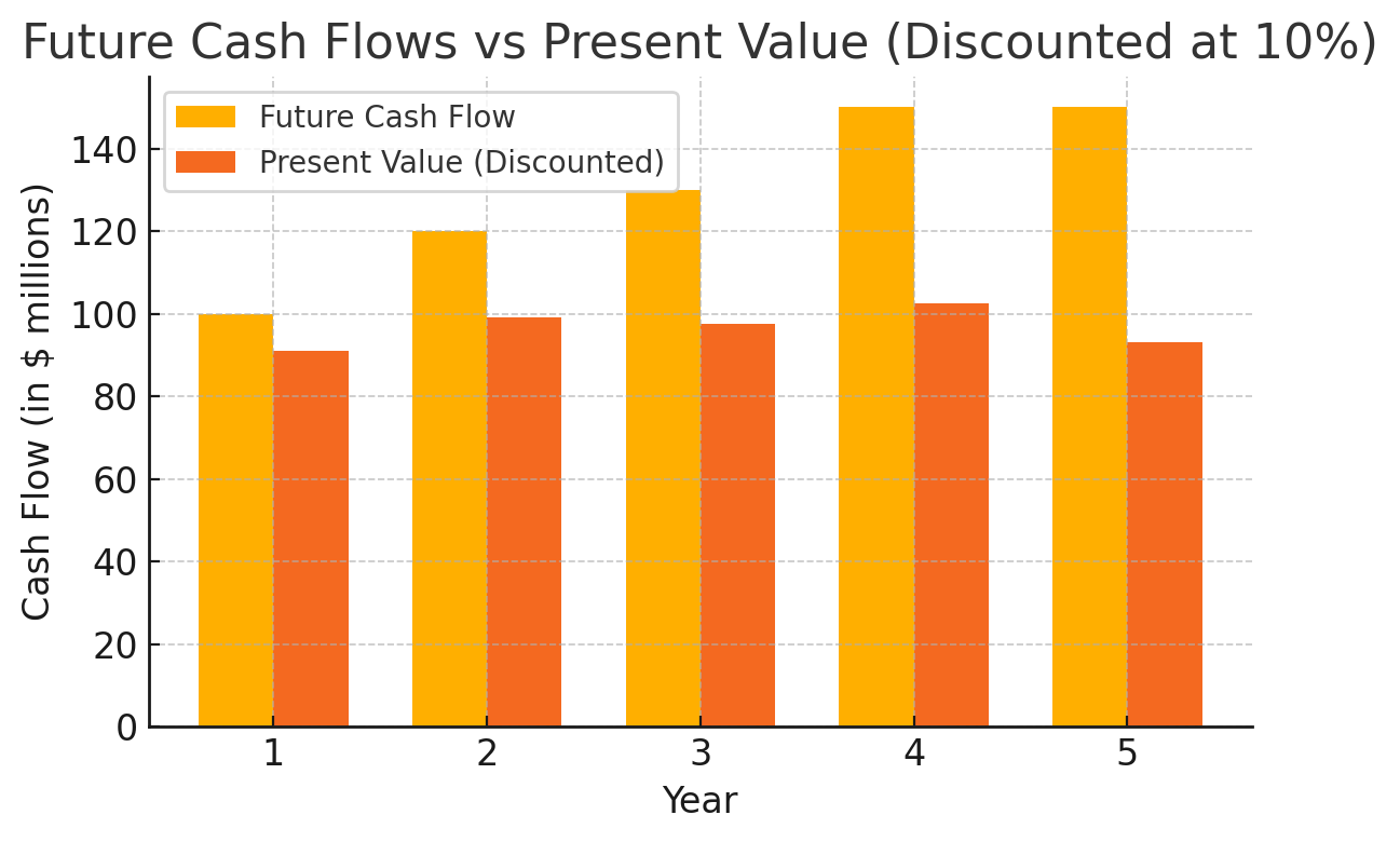
Figure: Illustration of DCF discounting – Future cash flows vs. their present value at a 10% discount rate. Even moderately distant cash flows (orange bars) are worth substantially less today (red bars) due to discounting.

The DCF approach is widely used as a starting point because it forces explicit assumptions about cash flow timing and risk. However, a plain DCF can be misleading in biotech. If one naively used a single high discount rate to “bake in” risk, the model may over-discount later cash flows. For example, using 40% for a Phase 1 project might appropriately penalize early years, but it also unduly slashes the value of potential late-stage revenues even if the drug succeeds.

The reality is that risk is not uniform over time – it decreases as milestones are met. Enter the next method: risk-adjusted NPV.

Risk-Adjusted NPV (rNPV) – Adjusting for Probability of Success

rNPV (also called eNPV, for “expected NPV”) builds on DCF by explicitly incorporating the probability of achieving each future cash flow. Instead of using one giant discount rate to cover all risks, rNPV uses a more moderate discount rate for time value of money and multiplies each cash flow by the probability it occurs. In formula form:

where P( t) is the probability the project hasn’t failed by time t. In practice, one assigns stage-specific success probabilities based on industry data (e.g. probability a Phase II trial succeeds, probability of FDA approval, etc.). Each future revenue or cost is risk-weighted by the chance the drug will make it that far. The result is an expected value reflecting both time value and technical risk.

Why go to this trouble? Because rNPV can more accurately reflect changing risk over a drug’s lifecycle. Early on, most drug projects have a <10% chance of ultimate approval. Under rNPV, most of the hefty Phase 3 revenues get multiplied by, say, 0.1, dramatically reducing their present value – but note this is conceptually different from just using a 40% discount rate. If the drug passes Phase I and II, its conditional probability of success might rise (say to 50%), and rNPV captures that updated value.

A plain DCF with a static discount rate “fails to reflect the decreasing risk over time”, whereas rNPV’s stage-by-stage probabilities do. In short, rNPV is the de facto standard for valuing individual biotech projects in industry because it handles binary risk more flexibly.

To illustrate, consider a Phase 1 oncology startup. Perhaps industry data says a Phase 1 oncology compound has ~10% chance of eventual approval. If projected peak cash flows in year 8 are $500 million, the DCF (with a high discount rate) and rNPV might mathematically yield similar values at t=0 if the discount rate was set to reflect 10% overall success odds.

But as time goes on, rNPV will step up the project’s valuation after each successful trial (since the failure probability drops out for that phase), whereas a static high discount rate would undervalue a de-risked Phase 3 asset. For this reason, pharma companies favor rNPV in portfolio valuations. In rNPV modeling, one must use credible probability data – fortunately extensive studies (e.g. BIO industry data) provide baseline success rates by phase and therapeutic area.

These can be adjusted if there’s reason to believe a project is above/below average (for example, if the drug targets a biologically validated mechanism, an investor might plug in higher-than-industry-average success odds).

After risk-adjusting cash flows, a lower discount rate (often 10–15%) is applied, since we’re not double-counting risk in the discount rate. In practice, large biopharma companies report using discount rates around 10% for rNPV analyses of R&D assets, much lower than the 20–30% VCs use for un-risk-adjusted DCF, because the risk is in the numerators now.

Takeaway

rNPV yields a more nuanced valuation that can bridge some understanding between optimistic founders and cautious investors. If a founder claims their project is worth $100 million because of huge future sales, an investor might counter that the risk-adjusted value is $10 million given the 10% success probability. rNPV lays that out in black and white.

Comparables and Precedent Transactions – The Market Lens

Not all valuations are built from scratch – often, “comparative valuation” is used, especially when public market or M&A data is available. The idea is to value the biotech based on how similar companies or assets are valued by the market. There are two main flavors:

Public trading comparables

Identify public biotech or pharma companies similar in stage, therapeutic area, or pipeline focus, and derive valuation multiples (e.g. enterprise value to revenue, EV to peak sales, or even EV per clinical asset). For example, if cancer immunotherapy biotechs trade at, say, 5× peak sales, and our startup’s drug could plausibly reach $200 M in annual sales, one might peg valuation around $1 B (5×$200 M), discounted for stage.

In early stages, revenue multiples might be swapped for R&D-based metrics – e.g. EV per Phase 2 asset in oncology, or comparing market caps of two companies each with a Phase 3 in the same indication.

Precedent M&A transaction

Look at prices paid in acquisitions or licensing deals for similar assets. In biotech, big pharma acquisitions provide rich data – e.g., the Kite Pharma deal (CAR-T therapy) at ~$12 B (toptal.com), or Pfizer’s 2023 acquisition of Seagen (an ADC oncology company) for $43 B (fticonsulting.com). These can be translated into implied values per drug or per indication. If another CAR-T startup has phase 2 data in a similar cancer, one might argue it’s worth a fraction of Kite’s price, adjusted for stage (Kite was later-stage).

Comparables are intuitively appealing (“if Company X is worth $Y, so are we!”), but use them with care. Biotech companies are highly idiosyncratic – differences in science or trial results can make direct comparisons misleading. Also, public market comparables can diverge from private deal valuations; public biotechs might be under- or over-valued due to market sentiment. As one Toptal analyst notes, “comparables…are often not applicable because most biotech companies are idiosyncratic” (toptal.com).

Still, comparables are a useful sanity check. For instance, if you’re valuing a Phase 3 orphan disease company and your DCF/rNPV comes to $500 M, but all five comparable public peers are trading at ~$300 M, that’s a signal to double-check assumptions (or to prepare to justify why you deserve a premium).

Likewise, knowing recent M&A multiples helps founders set realistic expectations – e.g. if similar Phase 2 assets sold for around $100 M upfront, it’s unlikely a VC will value your preclinical asset at $500 M unless there’s something truly extraordinary about it.

Metrics in practice: For established biotechs with revenues, traditional multiples like EV/Revenue or EV/EBITDA can be used (e.g. large profitable biotechs might trade at 4–8× revenue). But for earlier-stage, one sometimes uses EV per indication or EV per Phase X asset. Banks occasionally publish reports like “Phase 2 oncology deals average $X upfront, $Y total”.

These benchmarks feed into VC valuation heuristics. Ultimately, comparables anchor valuation in market reality – important for investors who plan an exit via IPO or sale and thus care about the eventual market pricing.

Venture Capital Method – Targeting the Exit and IRR

The Venture Capital (VC) method is a valuation approach specifically tailored to early-stage, high-risk companies where the focus is on the exit. It’s essentially a simplified DCF that only looks at the terminal value (exit proceeds) and applies a hefty discount (target return). In the words of one VC, the method is “a bastardized version of DCF…we take the projected exit value at the projected exit time and discount it” (medium.com).

Here’s how it works.

Estimate Exit Value: First, assume a scenario for the company’s value at exit. This could be an IPO market cap or an acquisition price in, say, 5–7 years. Often this is done by comparables as well – e.g. “If all goes well, in 5 years we could sell to Big Pharma for $500 M” or “IPO at $1 B”. The exit value is typically highly optimistic (because if the outcome is mediocre, the startup likely won’t exit at all). It’s not about average outcome; it’s about successful outcome value.

Determine Required Return (IRR)

VCs then decide what annual return they need for the risk. Early-stage biotech VCs often target 20–50% IRR (or more) on a successful deal. Higher risk and longer timelines push the required IRR to the upper end. For example, if a company is seed stage and very risky, a VC might demand the potential of a 50% annual return; for a more mature biotech, maybe 20–30%.

Discount the Exit Value to Present

Using the formula

the exit value is discounted back N years. This gives the post-money valuation today. (If new investment is about to be made, that present value is the post-money; if we want pre-money, subtract the new investment amount.)

Allocate Ownership:

The VC will invest such that their ownership %

Equivalently, they ensure that if the exit plays out as assumed, their equity stake will yield the target return. For instance, suppose a VC targets a 10× return in 5 years (which is ~58% IRR).

If they think a successful exit could be $500 M, they discount that at 58%/year:

If they invest $10 M now, that $50 M post-money means their $10 M buys 20% ownership (because $10 M is 20% of $50 M).

At exit, 20% of $500 M = $100 M, which indeed is 10× their $10 M. In practice, the VC might just say, “We’ll invest $10 M at a $40 M pre-money, $50 M post, to own 20%, aiming for a $500 M exit.” All numbers are negotiable, but that’s the gist.

The VC method is brutally outcome-focused. It often yields lower valuations than founders hope, because it bakes in both the probability of failure and the high opportunity cost of VC capital. Notably, the probability of failure isn’t always explicit in the formula, but it’s implicit in the high required IRR (the IRR is high partly because many portfolio companies will fail, so the winners must earn outsized returns).

As an analysis group piece described, differences in valuation approach (VC vs rNPV) can lead to big valuation gaps – e.g. a founder using rNPV might value a project at $50 M, whereas a VC using the target return method might value it at $20 M. Understanding this method helps founders realize where the other side is coming from: VCs are ultimately pricing in the exit potential and their desired “risk premium”.

One practical insight: time to exit is critical in the VC method. The longer the timeline, the more the discounting hurts. Biotech startups often face 5-10 year development timelines, which when combined with a 30-40% discount rate, shrink present valuations dramatically. Every extra year pushes the valuation down (since $(1+IRR)^N$ grows). Thus, demonstrating a credible plan to achieve value-inflecting milestones faster can improve the valuation.

Also, VCs typically assume dilution from future rounds in their calculations. For example, if they project a $500 M exit in 5 years but know the company will likely need another round, they may discount the exit further or target a larger ownership now to end up with a sufficient stake later. This is sometimes handled by assigning a higher required return to early rounds.

It’s a reality check against unbridled optimism. Founders should note that negotiation comes into play – valuations are ultimately a bargaining outcome, not just a formula. If you can show comparables indicating a higher exit or convince investors the risk is a bit lower, you might justify a better valuation. But if not, the VC method numbers will anchor the discussion.

Real Options Analysis – Valuing Flexibility and Strategic Choices

The real options method applies financial option pricing techniques to real-life investment decisions – in this case, drug development projects. The rationale: developing a drug is not an all-or-nothing straight line; at each stage (Phase 1, 2, 3, etc.) management has the option to continue or abandon. This flexibility has value. Traditional DCF or even rNPV treats the project in a static way, but real options valuation explicitly values the ability to make go/no-go decisions as uncertainties resolve.

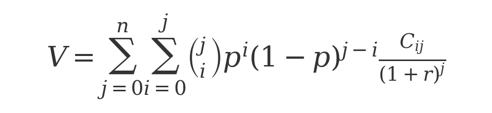
In effect, a biotech project can be seen as a series of call options: the Phase 1 investment gives you the right (but not obligation) to invest in Phase 2 if results are promising, and so on, up to the option to launch the drug. Real options analysis uses tools like decision trees, binomial lattices, or even Black-Scholes formulas to value these choices.

For example, imagine a biopharma has an opportunity to develop a new drug. It will cost $50 M in Phase 3 trials next year. If successful (say 60% chance), the drug is worth $500 M (NPV of cash flows); if it fails (40% chance), it’s worth $0. Management essentially holds an option to invest $50 M for a 60% chance at $500 M payoff. This looks like a call option with “underlying” $500 M, “exercise price” $50 M, and some probability distribution over outcomes. Using option valuation could yield, say, an option value of $X million.

Importantly, this value could be higher than a naive NPV which might simply do 0.6×$500 - 0.4×$50 = $something. Real options often increase the valuation of projects because they account for the downside protection of being able to abandon if things turn south. Management can cut losses, which asymmetrically improves the risk/reward (you invest only if promising, otherwise you stop spending – an option-like behavior).

Real options models in biotech can get complex. Typically, one constructs a lattice (binomial tree) of the drug’s estimated value through development milestones. At each node (e.g. after Phase 2 results), if the outlook is favorable, the company “exercises” the option to invest in the next phase; if not, it halts development (the option expires worthless, limiting further loss). This analysis requires inputs like the volatility of the project’s value – often estimated from stock volatility of comparable biotechs or using qualitative judgement (since project value volatility is not directly observable).

Higher volatility increases option value – an interesting twist, meaning risky projects might be worth more than their static NPV suggests if there is a chance of huge success and the ability to abandon failures.

(This aligns with intuition: biotech is a hits business, so having a “lottery ticket” pipeline with a few big winners and many failures can be rational if you can drop the failures quickly.)

Academic studies and some sophisticated corporate strategists use real options to evaluate R&D investments. In practice, real options is less commonly used by venture investors for day-to-day valuation, because it’s complex and relies on many assumptions. However, it provides valuable insight. For instance, it highlights the value of staged financing and partnerships: by investing in tranches or bringing in partners for expensive late-stage trials, companies are effectively exercising options selectively.

Real options thinking can also support higher valuations for platforms or portfolios: a biotech platform (e.g. an mRNA platform) might spawn dozens of drug “options,” which collectively are worth more than the sum of single-project NPVs.

In summary, real options analysis is the theoretical ideal for valuing biotech opportunities under uncertainty, capturing both upside volatility and managerial flexibility. It acknowledges that “the value of the drug’s future prospects is not fixed” and that the company can abandon or expand projects based on new information. If you ever see a valuation that seems surprisingly high for a pipeline, the team might be implicitly valuing real options (or just very optimistic!).

As a founder, understanding this approach can help in discussions with analytically minded investors – for example, you might argue that your lead program, while risky, is an option on a huge market, and the company can pivot or cut losses if early data disappoints (limiting downside). Such arguments, backed by real options logic, can justify a premium over pure rNPV in negotiations – provided the investors buy the assumptions.

Technical note

The real options method might involve using Black-Scholes-Merton formula or a binomial tree to value the option to continue at each stage. In a simplified scenario, one could treat a clinical-stage project like an option whose current “underlying asset” value is the NPV of cash flows if approved, the “exercise cost” is the remaining R&D cost, time to expiration is the development duration, and volatility is the uncertainty in project value. The output is a “real option value” higher than rNPV due to the option to abandon.

For the mathematically inclined, it’s a fascinating application of option pricing to corporate finance. For the less mathematically inclined – it reinforces a simple message: flexibility adds value. And conversely, anything that removes flexibility (e.g. a commitment that you must continue spending no matter what) reduces value.

Having surveyed these methods – DCF and rNPV as cash-flow models, comparables as market-based, VC method as return-based, and real options as flexibility-based – one sees that valuations can vary widely. It’s not uncommon for a founder using rNPV to claim a startup is worth $100 M while a VC using their method pegs it at $30 M.

The gap often comes down to risk adjustments and required returns. The best approach is often to triangulate – consider multiple methods and understand the drivers of each. For example, you might present an rNPV to show a rational, probability-weighted value, but also acknowledge the VC-method-implied valuation and comparables. This demonstrates to investors that you are realistic and not just drinking your own Kool-Aid. Conversely, investors who only use simplistic rules of thumb might miss the nuance that, say, your cancer therapy has a higher than typical Phase 2 success rate due to unique data – something an rNPV can highlight.

Before moving on, one practical aspect for founders to remember in equity valuation is the impact of dilution through fundraising and employee incentives. Biotech ventures typically go through multiple rounds of financing, and each round (plus the creation of stock option pools for employees) dilutes existing shareholders. By the time a biotech startup reaches a Series E or IPO, the founding team’s ownership might be in the single digits. (Data shows that after a Series E, founders often hold <10% of the company.)

This isn’t necessarily bad – 5% of a $1 B company is better than 50% of a $10 M company – but it underscores the importance of planning for dilution. Let’s discuss stock option pools and valuation next, as they bridge equity valuation and employee compensation.

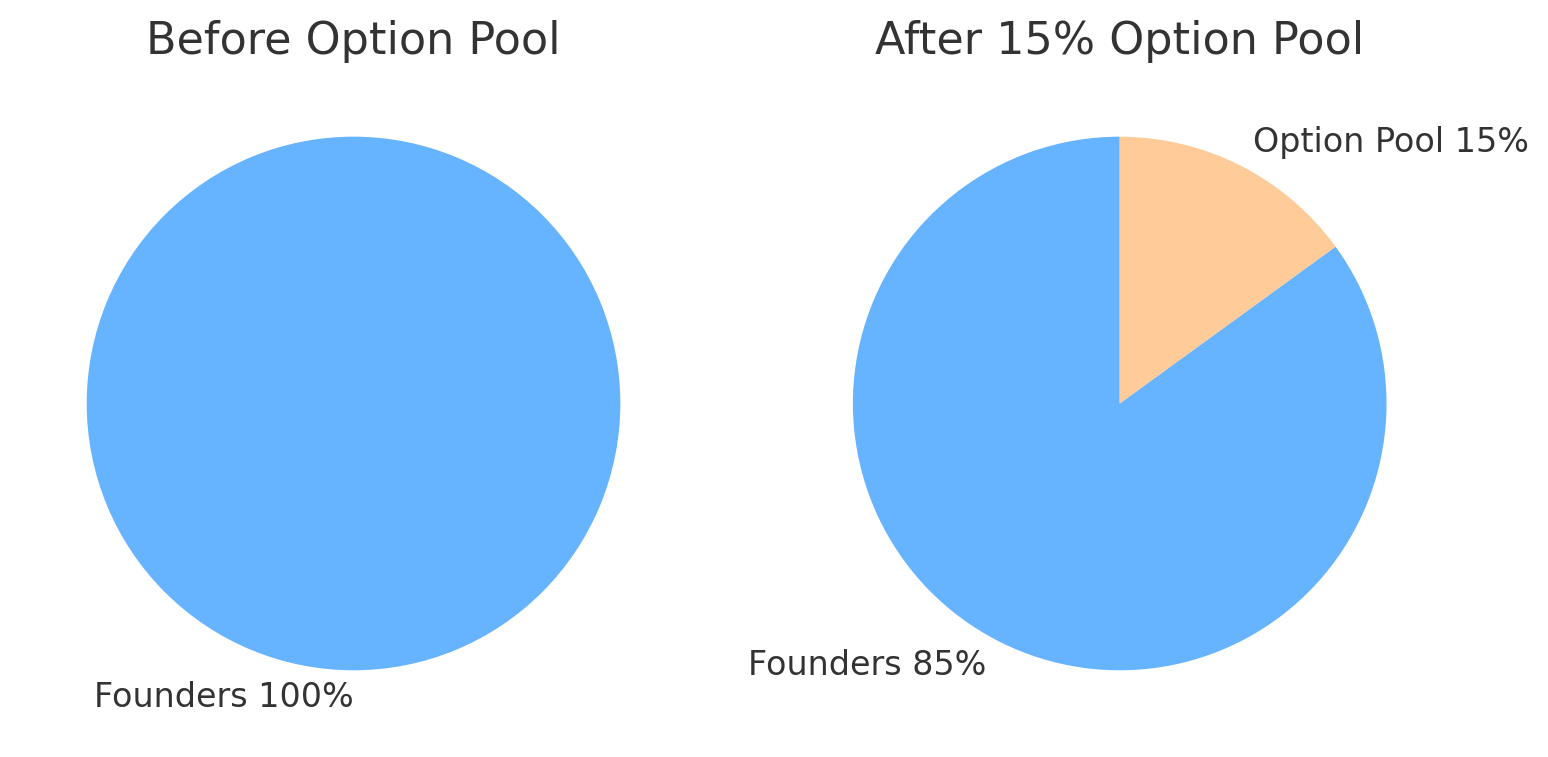
Figure: Cap table dilution from creating an employee option pool. In this example, founders owned 100% before. After setting aside a 15% option pool, founders own ~85% and the new pool accounts for 15%. An option pool is typically “carved out” of the pre-money valuation, meaning the dilution comes from the founders’ and existing investors’ slice.

Stock Option Valuation in Biotech (and Beyond)

Stock options are a crucial part of biotech compensation, especially for cash-strapped startups that need to attract talent. A stock option gives the holder the right (but not the obligation) to purchase shares at a fixed “strike” price, usually the market price at the time of grant (for private companies, the strike is often set at the 409A fair market value). If the company’s value grows, the option holder can eventually buy shares cheaply and either sell them (if liquid) or hold them, realizing a gain equal to the stock’s appreciation above the strike price.

From a valuation standpoint, a stock option is a derivative whose value derives from the underlying company’s equity value. Even if the option is at-the-money at grant (strike = current stock price, so intrinsic value is zero), it has significant time value – the possibility that the stock will be worth more in the future. Employees sometimes undervalue options because initially “it’s just the right to buy at today’s price”, but in reality that right can become very valuable if the company grows.

How do we quantify that value? Enter the world of option pricing models – chiefly, the Black-Scholes-Merton (BSM) model and binomial (lattice) models. These models, developed in financial economics, allow us to calculate a fair value of an option given certain assumptions. Public companies use them to expense stock-based compensation, and investors use them to value warrants and convertibles. Private venture-backed companies also use these models in 409A valuations and setting strike prices. Let’s break down the methods:

Black-Scholes Model – The Industry Standard Formula

The Black-Scholes-Merton model is the most famous formula for valuing options. Published in 1973, it earned a Nobel Prize for its creators and is widely used to this day. Black-Scholes provides a closed-form solution for the price of a European call option (one that can only be exercised at expiration) on a non-dividend-paying stock. The formula for a call option’s value (C) is:

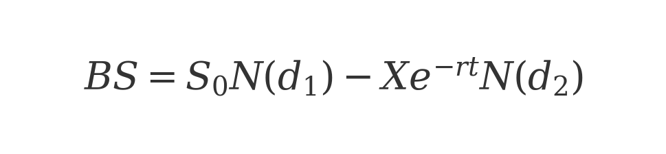
where So is the current stock price, K is the option strike price, T is the time to expiration (in years), $r$ is the risk-free interest rate, and N(d) is the cumulative normal distribution. The terms d1 and d2 are defined as:

with sigma being the volatility (standard deviation) of the stock’s returns. Don’t be alarmed by the math – in plain English, Black-Scholes says the option’s value = (stock * probability stock will finish in the money) minus (PV of strike * probability option will be exercised). The N(d) terms are those probabilities.

The five key inputs are: current stock price, strike price, time to expiration, volatility, and risk-free rate.

Intuitively: a higher current stock price S0 makes the option more valuable (already in the money); a higher strike K$ makes it less valuable; more time T increases value (more chance to eventually win out); higher volatility sigma greatly increases value (the more the stock can swing up, the more upside optionality – this is critical for startups); and a higher risk-free rate (r) increases call values slightly (because the present value of paying K at expiry is lower).

Black-Scholes assumes continuous trading, constant volatility and interest rates, and no dividends or early exercise, among other things.

Applying to startup equity

In practice, companies and valuation professionals use Black-Scholes to value employee stock options for accounting (ASC 718 / IFRS 2) and sometimes for setting an option’s exercise price discount. For a private biotech, you’d estimate sigma by looking at comparable public biotech stock volatilities (often high – e.g. 60-100% annualized), set T equal to the option’s expected life (more on this shortly), S0 based on the latest 409A valuation of common stock, K equal to that same value (if issued at FMV), and $r$ from Treasury yields.

The model then spits out a value per option, typically expressed as a percentage of the stock price. For example, a 10-year at-the-money option in a very volatile biotech might have a Black-Scholes value equal to, say, 60-70% of the stock price (meaning the option is almost as valuable as the stock itself because of the huge upside potential). Auditors accept Black-Scholes as the standard, because it’s well-understood and only requires a few parameters that can be objectively estimated (or at least agreed upon).

However, Black-Scholes has limitations when applied to employee stock options (ESOs). Notably, real employee options are American style (exercisable after vesting any time before expiration), and they have features like vesting periods, potential forfeiture if the employee leaves, and illiquidity (you can’t sell the option or hedge it).

Classic Black-Scholes doesn’t account for vesting or the inability to trade. It also assumes the option will be held to expiration if in the money, whereas employees often exercise early for various reasons (more on that soon). Despite these issues, companies often adjust inputs to approximate these factors. For example, they might use a shorter expected term in lieu of the full contractual term to reflect average early exercise behavior.

A common practice for options with a 10-year legal life is to assume an expected life of, say, 5–7 years based on historical data of when employees actually exercise (since many employees exercise soon after vesting or leave the company and have to exercise within 90 days). Using a shorter $T$ in Black-Scholes reduces the calculated value, which makes sense as forfeiture/early exercise reduces the upside time.

Let’s talk about those real-world adjustments in more detail.

Vesting

Employee options typically vest over several years. If an employee leaves before vesting, unvested options are forfeited (worth nothing). This effectively reduces the expected value compared to an immediately exercisable option. Valuers sometimes incorporate this by using an expected term that starts at the vesting date or by computing a “blended” expected life. Advanced models (like Monte Carlo simulations or forfeiture rate adjustments) can handle vesting explicitly, but Black-Scholes cannot.

Companies therefore may amortize the option expense over the vesting period and adjust for an estimated forfeiture rate of options due to turnover. From a pure value perspective, vesting lowers the option’s value to the employee (they might not stay to get it all), but from the company’s perspective, the expense is recognized over service as the option vests.

Illiquidity and Non-transferability

Unlike exchange-traded options, ESOs cannot be sold or easily cashed out before a liquidity event. This lack of marketability can reduce the practical value to holders. Some studies and practitioners apply an illiquidity discount to the Black-Scholes value. One approach (the Chaffee model) is to value a hypothetical put option that would insure the ESO’s value over the term – essentially, how much value is lost by not being able to sell. That put option cost becomes a discount to the ESO’s value.

For example, if a 5-year put costs 20% of the stock price, one might argue an untradeable option is worth 20% less than Black-Scholes says. Another simpler approach: assume employees will exercise as soon as they can sell (like right after an IPO lockup), effectively shortening the term. Indeed, empirical evidence shows employees exercise their stock options much earlier than expiration, often as soon as they are financially able or when they change jobs. Shorter holding periods reduce the option’s value.

Early Exercise and Employee Behavior

Employees are not the frictionless rational agents of the Black-Scholes world. They often exercise early because of risk aversion (their personal wealth is too tied up in the company), liquidity needs, or post-termination exercise deadlines (typically, if you leave a company, you have 90 days to exercise or the options expire). Early exercise means forfeiting some time value back to the company.

Many companies account for this by using the “expected term” approach as noted: e.g., if historical data or industry studies show employees on average hold options only ~5 years even though they have 10-year grants, the valuation will plug in $T=5$. This results in a lower option value than a full 10-year assumption, reflecting the reality that options get exercised or canceled sooner.

One academic study famously noted that Black-Scholes models without adjustment can overvalue long-dated employee options because they ignore things like mean reversion in stock prices and decreasing volatility as companies mature (business.columbia.edu) – whereas in reality, employees won’t all sit on options for 10 years if the company is doing well (they’ll cash out some) or doing poorly (the options will expire worthless or be underwater and likely forfeited).

Tax and Regulatory Differences (US vs EU)

The question specifically asks about EU/US differences. The core option valuation models (Black-Scholes, binomial) are universal, but the context and plan design can differ. In the US, stock options (especially Incentive Stock Options, ISOs) have favorable tax treatment but with conditions (like the $100K/year vesting limit for ISOs). In Europe, many countries historically did not embrace stock options to the same extent, although this is changing.

For example, broad-based option plans are far less common in Europe – only ~9% of European firms offer equity to more than 75% of employees, versus 33% in North America. European startups often face legal and tax hurdles: some countries tax stock option gains as salary (highly taxed), making them less attractive. Others have introduced special schemes (e.g. the UK’s EMI options, France’s BSPCE) that give tax advantages to startup options, trying to catch up with Silicon Valley norms.

From a valuation perspective, one practical difference is that in Europe, companies might use alternative long-term incentives like restricted stock units (RSUs) or phantom shares more frequently than US startups, because employees may perceive options as too risky or complicated. RSUs are simpler to value (essentially just the stock value, since an RSU is a promise of stock) but they lack the leverage of options.

The valuation of an option itself doesn’t change whether it’s in the US or EU – a Black-Scholes calculation is the same math in London or San Francisco. But the assumptions going in might differ. For instance, if European employees are more risk-averse and likely to exercise early or if local law forces a shorter exercise window, the expected term used might be shorter for an EU company’s option valuation than a comparable US company where employees might hold longer (though US employees also often face the 90-day post-termination rule unless companies extend it).

Additionally, differing interest rates (e.g. EU had negative rates in recent years) can slightly affect valuations (low $r$ increases the PV of the strike deduction, making options a tad cheaper, though this effect is usually minor relative to volatility).

In summary, Black-Scholes is the workhorse for option valuation – it’s generally accepted and easy to compute, but it must be adapted for the realities of employee stock options via adjusted inputs or complementary analysis. When precision is needed (for example, an option with performance vesting or market condition vesting), companies might turn to lattice models or Monte Carlo simulations.

Binomial (Lattice) Models – Handling Early Exercise and Complex Features

A binomial option pricing model uses a step-by-step lattice to value an option, which can naturally accommodate American-style exercise and other complexities. The idea is to model the underlying stock price moving up or down in discrete steps over the option’s life, and at each node, determine the option’s value by working backwards from expiration (dynamic programming). At each step, the option’s value is the discounted expected value of future payoffs or the payoff from early exercise, whichever is higher (for American calls with no dividends, usually it’s not optimal to exercise early, but for employee options, early exercise happens for extrinsic reasons as discussed).

Binomial models are often used in accounting for employee stock options when the options have vesting and the possibility of forfeiture. For example, FASB’s guidelines allow using binomial models to estimate fair value, and companies do so especially if the options have market conditions or other wrinkles that Black-Scholes can’t handle.

A lattice can incorporate assumptions about employee exercise behavior – e.g., one might input that employees will exercise if the stock reaches a certain multiple of the strike or after a certain time if in the money, to mimic how employees might behave. It can also model vesting by disallowing exercise in early nodes. The output is a more flexible model of option value.

When to use binomial models

If an option is straightforward (plain vanilla, time-based vesting, no performance conditions), Black-Scholes with an adjusted expected life is usually sufficient and preferred for simplicity. But if you have something like performance-based vesting (option only vests if a milestone is hit) or a cap on gains (some plans cap the payout), Black-Scholes fails to account for these.

A lattice can explicitly simulate the vesting condition – only allowing the option to exist in scenarios where performance is achieved – and thus give a more accurate value. Similarly, if trying to account for varying volatility over time (perhaps as a biotech moves from clinical to commercial stage, stock volatility might decline), a lattice can allow volatility to change at predefined points. Black-Scholes assumes constant volatility, which may not hold for a startup’s entire 10-year span (business.columbia.edu).

In practice, many valuation professionals will use a Black-Scholes model for most grants and occasionally a binomial model for unusual grants. For instance, say a biotech offers an option that expires early if the company doesn’t IPO in 5 years (a condition some companies used to attach). That early expiration conditional on an event is tricky for Black-Scholes but could be handled in a lattice.

The inputs for a binomial model are similar (stock price, volatility, etc.), but one also inputs assumptions on up/down movements per period or directly calibrates to match Black-Scholes (for consistency). The binomial will produce essentially the same value as Black-Scholes for a European option when using the same assumptions, but it enables valuation of American options – e.g., an American call with dividends or an American put, where early exercise can be optimal.

Employee options are American in form, but as noted, standard theory says it’s not rational to early-exercise a non-dividend-paying stock call from a value-maximization perspective. Employees do it for non-financial reasons, which we handle via custom assumptions.

Monte Carlo simulation is another method, often used for very complex payoffs (like path-dependent options). It involves simulating thousands of random stock price paths and averaging the option payoff, discounting back. For employee options, Monte Carlo is sometimes used if the vesting or payout depends on stock price hurdles (e.g. an option that vests only if the stock hits $X by year 3, etc.).

Putting It All Together for Stock Options

For a biotech founder/CFO, valuing stock options serves a few purposes:

• Determining the accounting expense (fair value at grant) and 409A valuation inputs.
• Understanding the real value being given to employees, to ensure equity comp is sufficient to motivate. For instance, if you issue options when your stock’s volatility is sky-high, the Black-Scholes value (and thus perceived value to a savvy employee) may be quite large even if strike == current price. If volatility later drops (say after an IPO), new option grants might be relatively less valuable. It’s important to calibrate how many options equal a meaningful reward.
• Setting expectations for employees: It can help to explain that a stock option’s value is not just stock price minus strike. There is time value which can be significant. This is why, for example, one often hears that an option grant of X number of shares is worth Y dollars in “option value” (which is much less than X * current stock price, unless deep in-the-money). Educating employees on the concept of risk/reward and time value can make them better appreciate the equity. Some companies even share the Black-Scholes value of grants with employees.

From a US vs Europe perspective, one also must consider how employees perceive options. In the US, especially in tech and biotech, employees are used to stock options and may value them highly (sometimes over-valuing them in their minds to be frank). In Europe, historically, many employees were more skeptical of options – partly due to fewer local success stories and less prevalence.

This is changing as European startup ecosystems mature and high-profile biotech exits occur. Still, a founder in Europe might need to spend more effort communicating the value of stock options to new hires (and potentially structuring grants in a more immediately tangible way, such as RSUs, if that’s more appealing locally). Also, European firms might lean on phantom stock or SARs (which cash-settle) in countries where issuing actual stock options is legally cumbersome. Those instruments would be valued similarly (they’re essentially options or units whose payoff equals the stock gain).

To summarize this section on stock option valuation:

• Black-Scholes: formula-driven, quick, standard. Great for most purposes, but assumes no weird features. We plug in an expected term (shorter than actual life if necessary) to account for early exercise/forfeiture. High volatility of biotech stocks means Black-Scholes values can be a large fraction of the stock price (biotech options are expensive, reflecting the huge uncertainty and upside).
• Binomial/Monte Carlo: more granular, used when we have vesting conditions, market conditions, or we want to directly model early exercise behavior. They provide a more custom-tailored valuation by simulating what could happen at each step.
• Adjustments: Illiquidity discounts or performance condition discounts are applied when relevant. For instance, if an option can’t be exercised until an IPO, and an IPO may never happen, one might treat that as a probability of zero payoff in certain scenarios, reducing value.
• EU vs US: The valuation math is the same, but usage patterns differ. US companies shower options on employees and thus have big option pools (15–20% is common), and employees have come to expect them. In Europe, option pools might be smaller and equity comp concentrated at higher levels (though this is slowly shifting). European startups might need to be mindful of different tax regimes (for instance, UK’s EMI options are highly efficient for employee and company if qualified). The overall cost of an option to a company (in terms of dilution and accounting expense) will be similar across borders for a given value, but the optics and uptake can differ.

Practical Tips for Founders

Valuation is both art and science, and it plays directly into how much of your company you give up and how you incentivize your team. Here are some actionable insights and tips for founders navigating biotech valuations and equity compensation.

Use Multiple Valuation Lenses

Don’t latch onto a single number. Consider running an rNPV and seeing what valuation the VC method would imply for the round. If you find huge divergence, be prepared to explain why (e.g., “Yes, our rNPV is $50 M, but we understand you need 3× return in 3 years, so you’d value it $15 M – perhaps we can structure milestones or tranches to bridge that gap”). Remember that valuations are ultimately negotiated, not handed down from a spreadsheet. Use data from all methods to inform your negotiation range.

Know Your Comparables

Even if you favor a DCF/rNPV approach internally, investors will ask “what are similar companies valued at?” If public comps or recent deals suggest a lower valuation than your model, address it head-on. Perhaps your science or IP is stronger – justify a premium with facts (e.g., “Unlike others, we already have Phase 2 data”). If comps suggest higher, use that to bolster your ask (“3 oncology biotechs with only preclinical assets sold for $100–200M; our $50M valuation is reasonable by comparison”). Being armed with comparables grounds your ask in market reality, which investors respect.

Understand the Investor’s Perspective

A VC looking at your startup likely has a target ownership and return in mind from day one. For example, a VC might say internally, “We need at least 20% ownership and a path to 10× on this deal.” This drives their valuation offer via the VC method. It’s helpful to reverse-engineer: given the size of investment you seek, what post-money valuation gives them that ownership? Does that align with any rational value of the company? If not, there’s a gap to reconcile. Perhaps you can negotiate a slightly smaller round or accept more dilution to reach a meeting point. Or consider structured deals: sometimes milestone-based tranches or warrants can effectively let the VC “pay up” for success (which is akin to embedding real options in the deal).

The Analysis Group paper noted that understanding different valuation approaches can help resolve differences between VCs and entrepreneurs. In practice, this might mean agreeing that if certain milestones are hit, the valuation steps up (a form of contingent valuation).

Plan Your Option Pool and Factor It I

Investor term sheets often require a pre-money option pool carve-out – e.g., “create a 15% option pool before we invest.” As shown earlier, this dilutes founders. Smart founders negotiate the pool size to avoid over-dilution. Think carefully about your hiring plan: how much equity do you really need to grant before the next round? If you can get away with a 10% pool instead of 20%, that difference is millions saved in founder equity. Also, time the pool creation strategically.

If you create a big pool and don’t use it fully before raising again, you essentially gave up equity for free. Investors will often include pool in the pre-money – you can counter by saying “we just hired key staff, we only need 5% more pool to reach next milestone.” Use data: typical pools at series A might be 10–15%. Don’t let a VC reflexively demand 20% if it’s not needed. It’s a point of negotiation.

Educate and Communicate with Your Team

In biotech, talent (scientists, execs) often join from academia or big pharma, and may not be familiar with startup equity’s value. Spend time explaining how stock options work, their potential upside, and also the risk. Be transparent that an option’s value is not guaranteed – it depends on the company’s success (aligning incentives). But also highlight success stories.

This is more crucial in cultures where equity comp isn’t the norm (e.g., a European hire who’s never had stock options might undervalue them). If needed, consider alternatives or sweeteners: some companies in Europe offer a choice of a slightly higher cash salary vs. more options, to accommodate risk preferences. As the CompTool survey indicated, outside the US many employees place greater value on cash or benefits. You might need to adjust your comp strategy country by country. But even in the US, ensuring employees truly understand the vesting schedule, exercise process, and potential tax implications (like AMT for ISOs, or ordinary income for NSOs) is part of being a good employer.

Equity vs. Salary Balance

For founders, your equity is your treasure. Use it wisely to incentivize, but don’t give it away needlessly. In biotech, top scientists or exec hires often expect meaningful equity – that’s fair. But structure grants with performance vesting if appropriate (e.g., a CSO gets additional option tranche upon successful IND filing) to align incentives.

If you’re in Europe or other regions where equity isn’t as valued, you might negotiate slightly lower option grants (relative to US norms) in favor of other comp forms – that can preserve your pool. Conversely, if someone really believes in the mission, they might accept more options instead of cash (happens often in US startups).

Dilution is Not (Always) the Enemy

A savvy founder realizes that raising capital at the right times, even if dilutive, increases the pie. Biotech is capital-intensive – you will likely go through multiple rounds. Plan your equity trajectory. If you start with, say, 50% as founder after seed, you might be 20% after Series B and <10% at IPO – this is normal. The key is to raise at increasing valuations (up rounds) so earlier dilutions are “worth it.” Sometimes, not raising (to avoid dilution) is penny-wise, pound-foolish – running out of cash or delaying trials can destroy value.

100% of zero is zero.

Better to own 10% of a company that cures cancer than 50% of a company that ran out of money in Phase 1.

Use your cap table projections alongside valuation assumptions to map out future dilution. When negotiating with VCs, if they insist on a low valuation, consider if taking more money to hit bigger milestones (reducing risk for next round) could justify it – sometimes a slightly worse deal now can lead to a much better one later if it means your Phase 2 data is rock-solid.

Leverage Non-Dilutive Funding When Possible

Especially in Europe, grants or public funding can boost value with no equity cost. If your biotech can get a €2 M Horizon grant or SBIR grant, that’s essentially an infusion that improves your rNPV (more cash, less dilution) and might let you negotiate a higher valuation in the next equity round. Be mindful though: too much reliance on grants can slow you down; VCs value speed to market. But non-dilutive money is a jewel – it can effectively increase the valuation pie for existing shareholders.

Prepare for Scrutiny on Option Valuations at IPO/Exit

If you’re eyeing an IPO, know that all those option grants you made will be looked at by auditors and possibly the SEC for cheap stock issues. Ensure your 409A valuations are done by reputable firms and reflect rising company value as you approach exit. Any large gaps (e.g. you granted options at $2/share FMV and 6 months later file for IPO at $10/share) will raise eyebrows.

Typically, valuation firms incorporate progress and comparables to steadily increase FMV. It’s both an art and science (again). As founder/CFO, be involved in that process to ensure integrity – you want to reward employees but not invite legal issues by artificially undervaluing grants.

Stay Witty but Wise

Maintain some wit and perspective. Valuations can feel like life or death, but ultimately they are a number on paper until an exit happens. Focus on building real value – successful trial results, IP, partnerships – because today’s valuation is just a waypoint. As one commentary put it, a startup’s paper valuation can make you a billionaire on Tuesday and back to nothing by Wednesday if the data fails. So use valuation as a tool, not an obsession. Negotiate hard but fair, take advice from mentors who have raised money before, and keep your eye on the prize: creating a biotech success story. If you do that, the valuations will eventually take care of themselves.

Conclusion

Valuing biotech equities and stock options involves blending analytical rigor with strategic narrative. By understanding DCF/rNPV calculations, speaking the language of VCs and comparables, and properly valuing your team’s stock options, you as a founder or finance leader can navigate the financial side of the biotech journey more effectively. Always cite your sources – whether it’s clinical data or valuation benchmarks – and approach negotiations armed with facts (and perhaps a dash of humor).

Remember that every valuation method is just a lens on the same underlying reality: the probability-weighted future of your biotech’s innovations. As the markets and your milestones evolve, so too will that valuation. So be prepared, be adaptable, and make sure everyone’s incentives – yours, investors’, and employees’ – are aligned toward the ultimate goal of saving patients’ lives and delivering returns. In the end, a clear-eyed approach to valuation is part of what turns a lab discovery into a thriving enterprise. Good luck, and may your molecule turn into a blockbuster!